[1] "numeric"[1] "character"After working through Tutorial 6, you’ll be able to…
Data types describe values. In R, we will most often encounter the following types of data:
| Data type | Description | Example |
|---|---|---|
| numeric | numbers used for calculations | c(1, 2, 3) |
| character | text strings | c("Green", "Yellow", "Blue") |
| factor | categorical variable with specific levels | education = factor(education, levels = c("low", "medium", "high")) |
| logical | logical values |
TRUE, FALSE
|
| NA | missing value | NA |
You can check a variable’s type using class().
Why do different data types matter? Many statistical functions require numeric input. Try, for example, to calculate mean of the following numbers:
Warning in mean.default(c("1", "2", "3")): Argument ist weder numerisch noch
boolesch: gebe NA zurück
[1] NAR will throw you an error message. Why? Because the values are stored as character strings, not as numeric values.
Character data requires quotations marks " to be recognized as such. See the difference here:
Missing values are stored as NA. You should always check whether values are missing (and of course, why).
Let’s check an example: We will again use the WoJ dataset. It contains a quantitative survey of N = 1,200 journalists from five countries, collected via the World of Journalism study. The data is provided via the tidycomm package developed by Unkel et al.
First, we retrieve the data and save it as an object named data_woj. Next, we count how many missing values exist in the variable work_experience. For this, we use three functions:
summarise(): reduces a dataset to a summary by computing statistics (for example counts or averages).sum(): adds values together. When used with logical values (TRUE / FALSE), it counts how many TRUE values exist - in this case, how many values are missing.is.na(): checks whether values are missing and returns TRUE for missing values and FALSE otherwise.library(tidyverse)
library(tidycomm)
data_woj <- tidycomm::WoJ
data_woj |>
summarise(n_missing = sum(is.na(work_experience)))# A tibble: 1 × 1
n_missing
<int>
1 13Most tidyverse functions allow handling missing values explicitly, using the na.rm() argument: Set it to TRUE if missing values (na) should be ignored (rm).
# A tibble: 1 × 1
   mean
  <dbl>
1  17.8
Now, imagine that you want to set specific values to NA. For example, we may want to set the value Freelancer in employment to missing. For this, we can use mutate, which we already know from previous tutorials, and na_if():
# Original data
data_woj |>
  head()
# A tibble: 6 × 15
country reach employment temp_contract autonomy_selection autonomy_emphasis
<fct> <fct> <chr> <fct> <dbl> <dbl>
1 Germany Nati… Full-time Permanent 5 4
2 Germany Nati… Full-time Permanent 3 4
3 Switzerla… Regi… Full-time Permanent 4 4
4 Switzerla… Local Part-time Permanent 4 5
5 Austria Nati… Part-time Permanent 4 4
6 Switzerla… Local Freelancer <NA> 4 4
# ℹ 9 more variables: ethics_1 <dbl>, ethics_2 <dbl>, ethics_3 <dbl>,
# ethics_4 <dbl>, work_experience <dbl>, trust_parliament <dbl>,
# trust_government <dbl>, trust_parties <dbl>, trust_politicians <dbl># Redefine missing values
data_woj |>
mutate(employment = na_if(employment, "Freelancer")) |>
head()# A tibble: 6 × 15
country reach employment temp_contract autonomy_selection autonomy_emphasis
<fct> <fct> <chr> <fct> <dbl> <dbl>
1 Germany Nati… Full-time Permanent 5 4
2 Germany Nati… Full-time Permanent 3 4
3 Switzerla… Regi… Full-time Permanent 4 4
4 Switzerla… Local Part-time Permanent 4 5
5 Austria Nati… Part-time Permanent 4 4
6 Switzerla… Local <NA> <NA> 4 4
# ℹ 9 more variables: ethics_1 <dbl>, ethics_2 <dbl>, ethics_3 <dbl>,
# ethics_4 <dbl>, work_experience <dbl>, trust_parliament <dbl>,
# trust_government <dbl>, trust_parties <dbl>, trust_politicians <dbl>Great, now you know all about types of data. While data types describe values, object types describe how values are stored.
As promised, this tutorial will also teach you about different types of objects:
| Object | Description | Example |
|---|---|---|
| scalar | single value | 3 |
| vector | multiple values of same type | c(1, 2) |
| tibble/data frame | collection of vectors | WoJ |
| list | collection of different objects | list(number = c(1,2), text = "word") |
| functions | a command that is to be computed | select() |
The “smallest” type of data you will encounter are scalars.
Scalars are objects consisting of a single value - for example, a letter, a word, a sentence, a number, etc.
You’ve already seen what a scalar looks like - remember when we started with R? Here, we defined an object word which only consisted of the word “hello”.
word <- "hello"
word
[1] "hello"Technically, scalars are vectors of length 1.
The next type of data you should know are vectors: Vectors contain multiple values of the same type. In tidyverse thinking:
Each column in a tibble is a vector.
A vector can only have one underlying type (e.g., numeric or character).
In principle, you can often (but not always) compare vectors with variables in data sets: They contain values for all observations in your data set (with all of these values being of the same data type).
An example would be the numbers from 1 to 20 that we worked with before. Now, it becomes apparent what the c() stands for - it specifies the vector format.
We define the object numbers to consist of the a vector c() which contains the values 1 to 20.
numbers <- 1:20
numbers
[1] 1 2 3 4 5 6 7 8 9 10 11 12 13 14 15 16 17 18 19 20We already know tibbles:
A tibble (or a data frame) combines several vectors of equal length.
Our data_woj data set from tidycomm is an example for this:
data_woj# A tibble: 1,200 × 15
country reach employment temp_contract autonomy_selection autonomy_emphasis
<fct> <fct> <chr> <fct> <dbl> <dbl>
1 Germany Nati… Full-time Permanent 5 4
2 Germany Nati… Full-time Permanent 3 4
3 Switzerl… Regi… Full-time Permanent 4 4
4 Switzerl… Local Part-time Permanent 4 5
5 Austria Nati… Part-time Permanent 4 4
6 Switzerl… Local Freelancer <NA> 4 4
7 Germany Local Full-time Permanent 4 4
8 Denmark Nati… Full-time Permanent 3 3
9 Switzerl… Local Full-time Permanent 5 5
10 Denmark Nati… Full-time Permanent 2 4
# ℹ 1,190 more rows
# ℹ 9 more variables: ethics_1 <dbl>, ethics_2 <dbl>, ethics_3 <dbl>,
# ethics_4 <dbl>, work_experience <dbl>, trust_parliament <dbl>,
# trust_government <dbl>, trust_parties <dbl>, trust_politicians <dbl>For a nice example for comparing scalars, vectors, and other data types check out this example here.
In R, we can access variables inside tibbles with the dollar sign $:
data_woj$countryWe can manually inspect the whole data frame using View():
View(data_woj)Finally lists:
Lists can store different object types of different lengths together.
As discussed, tibbles can include vectors consisting of different types of data (for instance, character and numeric vectors) but always of the same length.
In some cases, lists offer a more flexible way of saving very different objects within one object (i.e., the list).
Let’s check this example for a list:
As you see, the object includes three elements:
$data is the tibble data_woj
$numbers is the numeric vector numbers
$text is the character scalar text
across() to repeat operations over columns
When working with tibbles, you often want to apply the same operation to multiple variables at once. Instead of repeating the same command, you can use across().
across() allows you to apply one function (or several functions) to multiple columns simultaneously.
Suppose we want to transform all character variables to uppercase. We can do this like so:
# A tibble: 6 × 15
  country    reach employment temp_contract autonomy_selection autonomy_emphasis
  <fct>      <fct> <chr>      <fct>                      <dbl>             <dbl>
1 Germany    Nati… FULL-TIME  Permanent                      5                 4
2 Germany    Nati… FULL-TIME  Permanent                      3                 4
3 Switzerla… Regi… FULL-TIME  Permanent                      4                 4
4 Switzerla… Local PART-TIME  Permanent                      4                 5
5 Austria    Nati… PART-TIME  Permanent                      4                 4
6 Switzerla… Local FREELANCER <NA>                           4                 4
# ℹ 9 more variables: ethics_1 <dbl>, ethics_2 <dbl>, ethics_3 <dbl>,
#   ethics_4 <dbl>, work_experience <dbl>, trust_parliament <dbl>,
# trust_government <dbl>, trust_parties <dbl>, trust_politicians <dbl>You still have questions? The following tutorials & papers can help you with that:
Use the WoJ data. Save it as data_woj. Check the data type of the following variables:
countryemployment# A tibble: 6 × 2
country employment
<fct> <chr>
1 Germany Full-time
2 Germany Full-time
3 Switzerland Full-time
4 Switzerland Part-time
5 Austria Part-time
6 Switzerland Freelancer# A tibble: 1 × 2
country employment
<chr> <chr>
1 factor character Using data_woj…
work_experience.work_experience with NA.data_woj_clean.# A tibble: 1 × 1
n_missing
<int>
1 13# Replace values above 15 with NA
data_woj_cleaned <- data_woj |>
mutate(work_experience = replace(work_experience,
work_experience > 15,
NA))
# Check result
data_woj_cleaned |>
select(work_experience)# A tibble: 1,200 × 1
work_experience
<dbl>
1 10
2 7
3 6
4 7
5 15
6 NA
7 NA
8 11
9 NA
10 4
# ℹ 1,190 more rowsThis tasks contains several commands you do not yet know! Use data_woj (not the cleaned data set) and …
country_summary.trust_parliament, plot the average trust score!country_summary <- data_woj |>
group_by(country) |>
summarise(across(where(is.numeric), list(mean = ~ mean(.x, na.rm = TRUE),
n_miss = ~ sum(is.na(.x)))))
# Check the result
country_summary# A tibble: 5 × 23
country autonomy_selection_m…¹ autonomy_selection_n…² autonomy_emphasis_mean
<fct> <dbl> <int> <dbl>
1 Austria 3.92 0 4.19
2 Denmark 3.76 0 3.90
3 Germany 3.97 1 4.34
4 Switzerl… 3.92 0 4.07
5 UK 3.91 2 4.08
# ℹ abbreviated names: ¹autonomy_selection_mean, ²autonomy_selection_n_miss
# ℹ 19 more variables: autonomy_emphasis_n_miss <int>, ethics_1_mean <dbl>,
# ethics_1_n_miss <int>, ethics_2_mean <dbl>, ethics_2_n_miss <int>,
# ethics_3_mean <dbl>, ethics_3_n_miss <int>, ethics_4_mean <dbl>,
# ethics_4_n_miss <int>, work_experience_mean <dbl>,
# work_experience_n_miss <int>, trust_parliament_mean <dbl>,
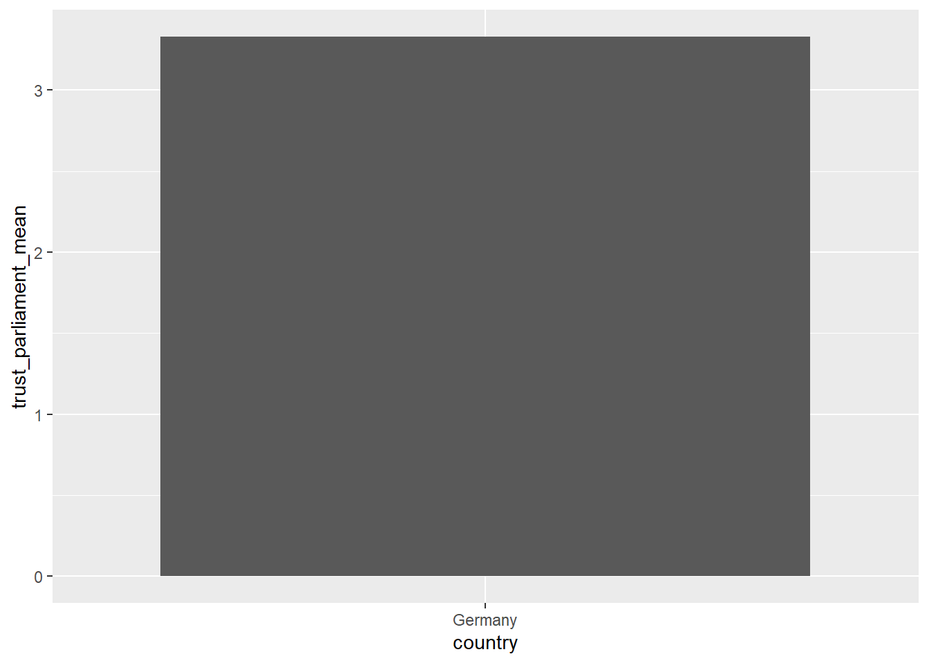
# trust_parliament_n_miss <int>, trust_government_mean <dbl>, …# For the country with the highest mean in `trust_parliament`, plot the average trust score!
country_summary |>
filter(trust_parliament_mean == max(trust_parliament_mean)) |>
# a very simple plot
ggplot(aes(x = country, y = trust_parliament_mean)) +
geom_col()